摘要

This application note describes the methods to minimize error in RTD temperature measurement.

Introduction

High-accuracy temperature measurements provide essential data for industrial automation applications to ensure both product quality and safety. Many types of temperature sensors are available, and each one has its advantages and disadvantages. This application note focuses on resistance temperature detectors (RTD), and explains the design essentials to optimize the measurement accuracy.

Resistance Temperature Detectors

RTDs contains an element whose resistance changes with temperature. Most elements are either platinum, nickel, or copper. A platinum RTD provides the best performance because platinum has the most linear and repeatable temperature-to-resistance relationship over a large temperature range.

Generally, RTDs generate more stable and repeatable outputs, compared to thermocouples and thermistors. Hence, RTDs achieve higher measurement accuracy.

High-Accuracy RTD Measurement Design Options

The two most common methods to measure an RTD are constant current excitation (Figure 1) and constant voltage excitation (Figure 2).

The goal is to accurately measure the RTD resistance and convert it to temperature using an equation or a lookup table. For ideal cases:

for constant current excitation,

or

for constant voltage excitation.

However in practice, the lead wires of the RTD have resistance. Long lead wires greatly affect the measurement accuracy. Therefore, the actual resistance measured by the circuits shown in Figures 1 and 2 is:

RTD + (2 × R_WIRE),

where R_WIRE is the resistance of the lead wires, assuming both wires have the same resistance. Although theoretically acceptable, the same R_WIRE implies that both wires are of the exact same length and made with the exact same material. Such an assumption cannot be guaranteed in critical temperature sensing applications. For this reason, RTDs feature 3-, and 4-wire configurations to help eliminate the measurement error contributed by lead wires.

3-Wire RTD Configuration

Typical constant current and constant voltage excitation circuits for 3-wire RTD are shown in Figure 3 and Figure 4, respectively. In both cases, the ADC samples a resistance of RTD + R_WIRE3 (where R_WIRE3 is the resistance of the return lead wire). The system eliminates R_WIRE2 because the ADC inputs are typically high-impedance and virtually no current flows through R_WIRE2. Therefore, the ADC only measures the voltage across RTD and R_WIRE3. R_WIRE3 contributes to measurement error. Compared to 2-wire configuration, however, the error contributed by the lead wires are reduced by roughly 50%.

One method to further improve the measurement accuracy is by adding an analog switch to the circuit. The ADC then measures the voltage (V_X) at the output of the excitation signal and obtains a value for R_WIRE1. By assuming R_WIRE1 is approximately the same as R_WIRE3, the R_WIRE3 can be subtracted out. Referring to Figure 3, in current excitation configuration, R_WIRE1 resistance equals to:

And, the improved approximation of the RTD resistance is:

For voltage excitation configuration:

and

This method to improve the measurement accuracy does require extra hardware and adds complexity to the software.

4-Wire RTD Configuration

A 4-wire RTD configuration provides the highest measurement accuracy. Figure 5 and Figure 6 show the constant current excitation and constant voltage excitation circuits, respectively, for 4-wire RTD. For current excitation configuration,

because no current passes through R_WIRE2 or R_WIRE3. Therefore, the voltage across R_WIRE2 + RTD + R_WIRE3 is the same as the voltage across the RTD. Unfortunately, when using a constant voltage excitation configuration, because of the voltage divider effect, R_WIRE1 and R_WIRE4 still creates errors in the RTD measurement unless the ADC system has the ability to measure the voltage at the excitation voltage output (V_X). If the voltage at V_X is known, then the reference current can be calculated by

where R_REF is 3.32kO in this case. Similarly,

is the same as the formula for the current excitation configuration.

Many other factors in the signal chain affect the accuracy of measurement. These factors include the input impedance of the ADC system, the resolution of the ADC, the amount of current through the RTD, the stability of the voltage reference, and the stability of the excitation signals.

The inputs of the ADC system must be high impedance to avoid voltage drops across the lead wires (R_WIRE2 and R_WIRE3 in 4-wire configuration for example). If the ADC doesn't have high impedance inputs, buffers should be added in front of the inputs of the ADC.

Heating Error

Although an RTD is a sensor, it is also a resistor. When current passes through a resistor, there is power dissipation. The dissipated power heats up the resistor. This self-heating effect creates error in the measurement. Excitation current must be carefully chosen to ensure the error created is within the error budget. The key formula to calculate the self-heating error is

ΔT = (I²_REF ×R_RTD) × F,

where F is the self-heating factor of RTD, expressed in mW/°C. For example, a PT-100 platinum RTD with a 0.05°C/mW self-heating factor submerged in ice water. When the measuring temperature is 0°C, R_RTD equals to 100Ω. If the I_REFis set to 10mA, the self-heating error becomes

((0.01A)² × 100Ω) × 50°C/W = 0.5°C.

Depending on the application, this error may or may not be acceptable. For high-accuracy measurements, a lower excitation current reduces the self-heating error. For example, if I_REF is lowered to 1mA, the self-heating error becomes 0.005°C. This level of error is much more tolerable. While reducing the excitation current reduces the self-heating error, it also reduces the voltage signal span across the RTD, thus requiring the RTD signal to be amplified so that the ADC can extract more discrete signal levels. An alternative would be to use a higher resolution ADC.

Up to this point, all the formulas discussed involve either I_REF or V_REF. But, what if these excitation signals are not stable? Instability can result from short term or long-term drift. Clearly, if the excitation signals become inaccurate, all the calculations above have errors. Consequently, periodic calibrations are required. Of course, an engineer could use a super stable voltage reference with ultra-low temperature drift and long-term drift. However, usually such devices are very costly. Alternatively, the ratiometric temperature measurement method eliminates errors caused by inaccurate excitation signals.

Ratiometric Temperature Measurement

A ratiometric measurement provides measurement of the resistance of the RTD as a ratio of the reference resistance, instead of measuring the resistance using an absolute voltage. In other words, R_RTD will be a function of R_REF instead of V_REF or I_REF. This uses the same excitation signal to generate both the voltage across the RTD and the voltage reference for the ADC. When the excitation signal changes, that change is reflected on both the voltage across the RTD and the reference inputs of the ADC. Figure 7 and Figure 8 show the ratiometric measurement circuits for current excitation and voltage excitation configurations.

The general ADC conversion formula is:

where

V_IN = ADC input voltage
V_REF = reference voltage (REFP - REFN)
CODE = ADC code
N = resolution of the ADC.

V_IN equals the voltage across the RTD. For current excitation mode

V_IN = I_REF × R_RTD and V_REF = I_REF × R_REF.

Substituting V_IN and V_REF into the ADC conversion formula yields,

and subsequently,

Similarly for voltage excitation,

Substituting V_IN into the ADC conversion formula yields,

Solving for R_RTD gives,

In both cases, after the simplification, R_RTD becomes a function of R_REF and ADC code; hence, the accuracy of the RTD measurement depends on R_REF. For this reason, when selecting a reference resistor, the engineer must pick one with low temperature and long-term drift.

RTD to Temperature Conversion

No matter how well the circuit measures the resistance of the RTD, all efforts are wasted if the engineer does not have a good method to accurately convert RTD resistance to temperature. One common method is to use a lookup table. However, if the resolution requirement is high and the measuring temperature range is wide, the lookup table becomes unwieldy, and the method less effective. Another method is to calculate the temperature.

For a platinum RTD, the Callendar-Van Dusen equation describes the relationship between resistance and temperature as:

R(t) = R0 × (1 + A × t +B × t² + (t - 100) × C × t³),

where

R(t) = RTD resistance
t = temperature
R0 = resistance of the RTD at 0°C
A = 3.908 × 10^-3
B = -5.775 × 10^-7
C = -4.183 × 10^-12 when t < 0°C
C = 0 when t > 0°C

This equation provides the expected RTD resistance given a known temperature. If the temperature range of interest is above 0°C, then the constant C becomes 0 and the equation becomes a quadratic formula. Solving a quadratic equation is straightforward. But, if the temperature goes below 0°C and the C constant becomes non-zero, the equation becomes a difficult 4th order polynomial. In this case, polynomial interpolation approximation is a very useful tool. Here is a Microsoft Excel solution:

1. On a spreadsheet, create two columns of data. One column lists the temperature. The second column lists the corresponding RTD resistances calculated from the Callendar-Van Dusen equation.
2. Create an X-Y scatter plot.
3. Add a polynomial trendline for the plot. A higher order of the polynomial gives a more accurate approximation.
4. Select "Display Equation on Chart" in the "Format Trendline" menu.

The resulting polynomial equation for a PT100 for t < 0°C is:

t = -1.6030e -13 × r⁶ + 2.0936e -10 × r⁵ -3.6239e -8 × r⁴ -4.2504e -6 × r³ + 2.5646e -3 × r² + 2.2233 × r -2.4204e2

Increasing the decimal places of the polynomial coefficients reduces error. With four decimal places, as shown in the formula above, the temperature approximation error is less than 0.005°C, tolerable for most applications.

Maxim Reference Design Solution

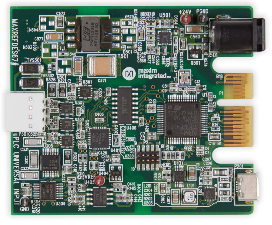
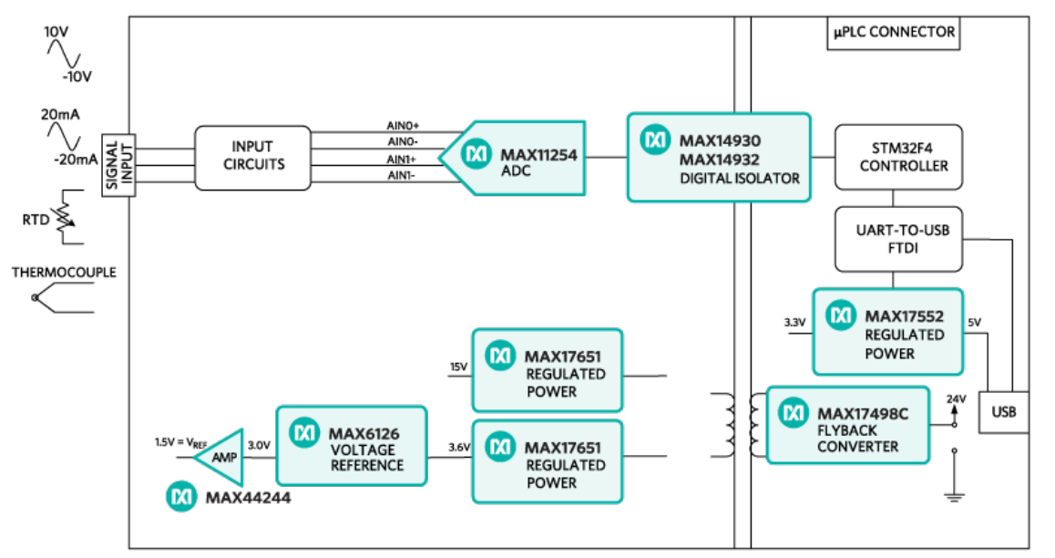
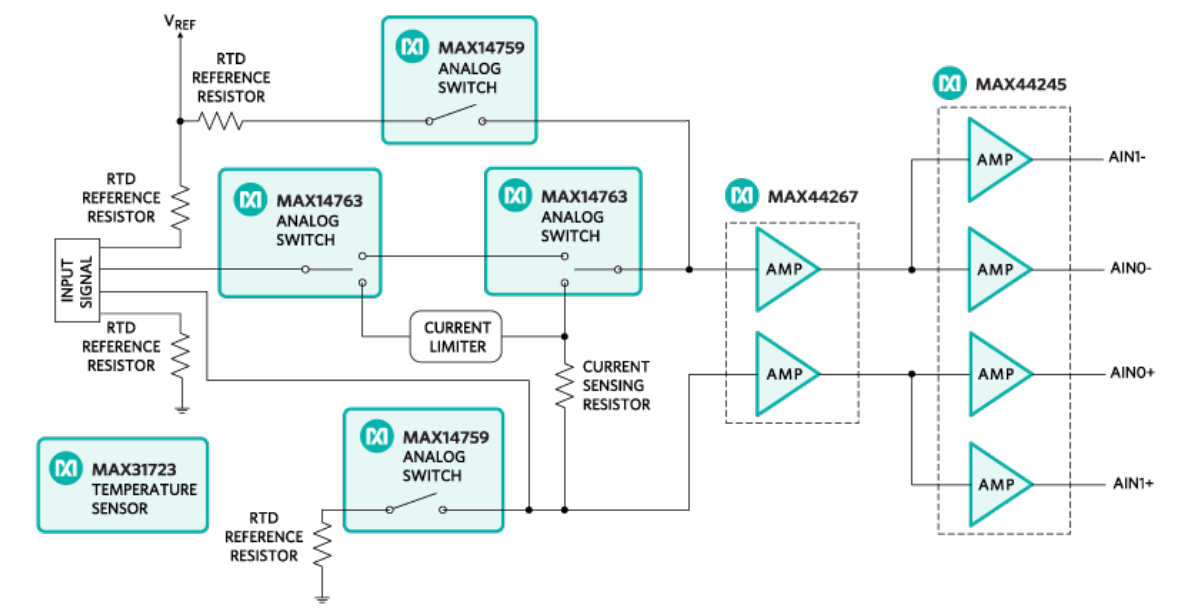
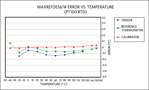
MAXREFDES67# reference design implements the 4-wire ratiometric configuration and polynomial approximation, as described above. In addition, design files and firmware are available for subsequent modification and implementation. Furthermore, this reference design (Figures 9, 10, 11) is a complete universal analog input for industrial applications. Besides RTD measurement, this unique 24-bit front-end also accepts bipolar voltage and current, and thermocouple (TC) inputs. Built in Maxim Integrated's ultra-small Micro PLC form factor, the MAXREFDES67# performs with an effective resolution up to 22.3 bits with temperature error as low as ±0.1% across a range of -40°C to 150°C. Figure 12 shows the temperature error measured by the MAXREFDES67# RTD input versus temperature referenced to three different thermometers. The references are the Omega HH41 thermometer, the ETI reference thermometer, and Fluke 724 temperature calibrator, respectively. The MAXREFDES67# connected RTD probe (Omega P-M-1/10-1/4-6-0-G-3) was placed in the Fluke 7341 calibration bath and calibrated at 20°C.

Conclusion

Temperature is the most measured industrial parameters. Though precision system design using techniques like the ratiometric method and polynomial approximation make very accurate measurement systems, with Maxim's reference design system, designers can now develop high-accuracy RTD temperature measurement or thermocouple measurement systems faster than ever before. The MAXREFDES67# allows modification and implementation, and is a complete universal analog input for industrial applications. Besides RTD measurement, it also accepts bipolar voltage, current and thermocouple inputs, performs with an effective resolution, and low measurement error making it more effective than other options.

A similar version of this application note appeared February 2016 on EDN Network.