pH Sensor Reference Design Enabled for RF Wireless Transmission
Designing wireless data transmission from a sensor node for remote monitoring is a considerable challenge if system accuracy, efficiency, and reliability are critical. The pH level of a solution is one of the measurements often considered in many industries, such as in agriculture or in the medical field. The main objective of this article is to evaluate the characteristics of a pH glass probe in order to address the different challenges in hardware and software design, and to present a solution for wireless data transmission from the probe using a radio frequency transceiver module.
Introduction
The first part of this article addresses the pH probe, which is followed by an examination of the different design challenges related to the front-end signal conditioning circuit and how to achieve a low cost with high precision and reliability in data conversion. As a method to increase the accuracy and precision in data processing, calibration techniques such as a general polynomial fit using the least square method for approximation in scattered predefined data for pH calibration will also be included in the discussion. The last part of this article provides a reference circuit design for a wireless monitoring system.
Understanding the pH Probe
pH Defined
An aqueous solution can fall under acidic, alkaline, or neutral levels. In chemistry, this is measured by a numeric scale, called pH, which stands for power of hydrogen according to the Carlsberg Foundation. This scale is logarithmic and goes from 1 to 14. The pH level can be express mathematically as pH = –log(H+). Therefore, if the hydrogen ion concentration is 1.0 × 10⁻² moles/liter, then pH = –log(1.0 × 10⁻²) gives a value of 2. An aqueous solution like distilled water has a pH value of 7, which is a neutral value. Solutions with a pH value below 7 are acidic, while those above a pH value of 7 are considered an alkaline solution. The logarithmic scale gives a degree of the acidity of a solution as compared to another.
For example, a solution with a pH value of 5 is 10 times more acidic than a solution with a pH value of 6, and 1000 times more acidic than a solution with a pH value of 8.
pH Indicators
There are many ways to measure the pH level of an aqueous solution. This can be done through a litmus paper indicator or through the use of a glass probe.
Litmus Paper
A litmus paper indicator is usually made up of dyes extracted from lichens that serve as a pH level indicator. Once in contact with a solution, the paper has a chemical reaction that results in a change in color that indicates the pH level. This category basically includes two methods: One involves comparing the standard color corresponding to a known pH with the color of an indicator immersed in the test liquid using buffer solution, and the other method involves preparing pH test paper that is soaked in the indicator, then immersing the paper in the test liquid and comparing its color with the standard color. Though the two mentioned methods are easy to implement, they can be prone to errors resulting from temperature and foreign substances in the test solution.
pH Glass Probe
The most commonly used pH indicator is a pH probe. It consists of a glass measuring electrode and a reference electrode. A typical glass probe is made up of a thin glass membrane that encloses a hydrogen chloride (HCl) solution. Inside the enclosure is a silver wire coated with AgCl, which acts as a reference electrode that is in contact with the HCL solution. The hydrogen ions outside the glass membrane diffuse through the glass membrane and displace a corresponding number of sodium ions (Na+), which are normally present in most glasses. This positive ion is subtle and confined mostly to the glass surface on whichever side of the membrane has the lower concentration. The excess charge from the Na+ generates a potential voltage at the sensor output.
The probe is analogous to a battery. When the probe is placed in a solution, the measuring electrode generates a voltage depending on the hydrogen activity in the solution, which is compared to the potential of the reference electrode. As the solution becomes more acidic (lower pH value) the potential of the glass electrode becomes more positive (+mV) in comparison to the reference electrode, and as the solution becomes more alkaline (higher pH value) the potential of the glass electrode becomes more negative (−mV) in comparison to the reference electrode. The difference between these two electrodes is the measured potential. A typical pH probe ideally produces 59.154 mV/pH units at 25°C. This is usually expressed by the Nernst equation as shown below:
Where:
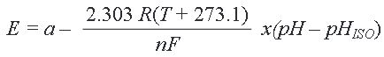
E = voltage of the hydrogen electrode with unknown activity
a = ±30 mV, zero point tolerance
T = ambient temperature in 25°C
n = 1 at 25°C, valence (number of charges on ion)
F = 96485 coulombs/mol, Faraday constant
R = 8.314 volt-coulombs/°K mol, Avogadro’s number
pH = hydrogen ion concentration of an unknown solution
pHISO = 7, reference hydrogen ion concentration
The equation shows that the voltage generated is dependent on the acidity or alkalinity of the solution and varies with the hydrogen ion activity in a known manner. The change in temperature of the solution changes the activity of its hydrogen ions. When the solution is heated, the hydrogen ions move faster, which results in an increase in potential difference across the two electrodes. In addition, when the solution is cooled, the hydrogen activity decreases causing a decrease in the potential difference. Electrodes are designed ideally to produce a zero volt potential when placed in a buffer solution with a pH value of 7.
A typical pH probe would have a specification as shown in the following table:
| Measurement Range | pH 0 to pH 14 |
| pH at O V | pH 7.00 ±0.25 |
| Accuracy | pH 0.05 in the range from 20°C to 25°C |
| Resolution | pH 0.01 0.1 mV |
| Operating Temperature | Maximum 80°C |
| Reaction Time | ≤1 sec for 95% of final value |
A pH probe plays an important role in this study since data reliability will depend on the sensor’s accuracy and its stability. Two keys factors that will be considered in choosing a pH probe are its stability time after a temperature change and its stability time after a change in the buffer solution pH value. As an example, the data taken from Jenway’s application note, “An Evaluation of Jenway Performance pH Electrode”1 the performance of the probe at a given test condition in testing its stability after a temperature change. A liquid solution having pH 7 @ 20°C and pH 4 @ 60°C buffers were prepared and each electrode was allowed to stabilize in the pH 7 buffer stirred at 200 rpm. The electrode was then rinsed with deionized water and transferred to the aliquot of pH 4 buffer for a period of 4 minutes. The electrode was again rinsed with deionized water and returned to the pH 7 buffer. The time taken for the reading to remain stable for 10 seconds was then assessed. The test was repeated in triplicate for each probe.
| General-Purpose pH Probe | Jenway (35xx Series pH Probe) | |
| 1 | 77 | 36 |
| 2 | 77 | 33 |
| 3 | 49 | 34 |
| Mean | 67.6667 | 34.3333 |
| General-Purpose pH Probe | Jenway (35xx Series pH Probe) | |
| 1 | 29 | 21 |
| 2 | 31 | 26 |
| 3 | 38 | 21 |
| Mean | 32.6667 | 22.6667 |
Jenway’s performance compared to a general-purpose pH probe shows a difference of up to 50% faster in response within the given conditions shown above. Using an instrument like this will benefit greatly from reducing the time required in analyzing the data because of its high throughput of samples.
Sensor Analog Signal Conditioning Circuit
It is important to understand the equivalent electrical diagram of the sensor probe in order to arrive at an appropriate signal conditioning circuit. As described in the previous section, the pH probe is made up of glass that creates an extremely high resistance that can range from 1 MΩ to 1 GΩ and acts as resistance in series with the pH voltage source as shown in Figure 1.


Even a very small circuit current traveling through the high resistances of each component in the circuit (especially the measurement electrode’s glass membrane), will produce relatively substantial voltage drops across those resistances, seriously reducing the voltage seen by the meter. Making matters worse is the fact that the voltage differential generated by the measurement electrode is very small, in the millivolt range (ideally 59.16 millivolts per pH unit at room temperature). The meter used for this task must be very sensitive and have an extremely high input resistance.
Analog-to-Digital Conversion
For this type of application, given the response time of the sensor, the sampling rate for data gathering will now be an issue. With a given sensor resolution of 0.001 V rms and an ADC full-scale voltage range of 1 V, a high resolution ADC will not be required to achieve an effective resolution of 9.96 bits. Noise free resolution is defined in units of bits with the equation: Noise free resolution = log2 [full-scale input voltage range/sensor peak-to-peak voltage output noise]. The sampling rate of the ADC can be a great factor for low power application since the ADC’s sampling rate is directly related to its power consumption. So given the response time of the sensor, the typical ADC sampling rate can be set into its lowest throughput. A microcontroller with an integrated ADC can be used to reduce component count.
Transceiver
Transmitting pH and temperature data requires a transceiver, and controlling a transceiver requires a microcontroller. Choosing both the transceiver and microcontroller involves some key considerations.
Choosing a transceiver involves few considerations that must be taken into account:
- Operating frequency
- Maximum distance range
- Data rate
- Licensing
Operating Frequency
In designing RF transmission, the operating frequency (OF) must determine if a sub-GHz or 2.4 GHz frequency will serve the application requirement. In an application that requires a high data rate and uses wide bandwidth like Bluetooth, the 2.4 GHz frequency is the best choice to use. But when the application is industrial, a sub-GHz will be used because of the available proprietary protocols that readily provide the link layer of the network. ISM frequencies in the sub-GHz range that proprietary systems primarily use are 433 MHz, 868 MHz, and 915 MHz.
Maximum Distance Range
Sub-1 GHz frequencies offer long range capability that can accommodate high power and reach over 25 km. These frequencies, when used in simple point-to-point or star topology, can effectively pass through walls and other barriers.
Data Rate
The data rate also needs to be determined as it affects the transmission distance capability and power consumption of the transceiver. A higher data rate consumes less power and can be used over a short distance while a lower data rate consumes power and can be used in long distance transmission. Increasing the data rate is a good method for improving power consumption as it only draws bursts of current from the battery in short periods of time, but this also reduces the distance of radio coverage.
Transceiver Power Consumption
Transceiver power consumption is important for battery-powered applications. This is also a factor in many wireless applications because it dictates the data rate and distance range. The transceiver has two power amplifier (PA) options to allow greater usage flexibility. The single-ended PA can output up to 13 dBm of RF power and the differential PA can output up to 10 dBm. For illustration, Table 4 shows a summary of some of the PA output powers vs. transceiver IDD current consumption. For completeness the receive mode current consumption is also shown.
| Transceiver State (868 MHz/915 MHz) |
Output Power (dBm) | Typical IDD (mA) |
| Single-Ended PA, Tx Mode |
–10 0 +10 +13 |
10.3 13.3 24.1 32.1 |
| Differential PA, Tx Mode |
–10 0 +10 |
9.3 12 28 |
| Rx Mode | - | 12.8 |
Licensing
Sub-GHz includes license-free ISM bands at 433 MHz, 868 MHz, and 915 MHz. It is widely used in industrial and highly suitable in a variety of wireless applications. It can be used in different regions of the world because this complies with the European ETSI EN300-220 regulation, the North American FCC Part 15 regulation, and other similar regulatory standards.
Microcontroller
As shown in Figure 2, the heart of RF systems is a processor unit or microcontroller (MCU) that processes data and runs software stacks interfaced to a transceiver for RF transmission and to a pH reference design (RD) board for sensor measurement.


Choosing a microcontroller involves few considerations that must be taken into account:
- Peripherals
- Memory
- Processing power
- Power consumption
Peripherals
A microcontroller should be integrated with peripherals like an SPI bus. The transceiver and the pH reference design board are connected via SPI and therefore two SPI peripherals are required.
Memory
With a decent amount of memory, a microcontroller is where protocol processing and sensor interfacing takes place. Flash and RAM are two very critical components of microcontrollers. To make sure that the system won’t run out of space, 128 kB were used. These undoubtedly make application and software algorithms run smoothly and this will give room for possible upgrades and added functionality, which make the system headache free.
Architecture and Processing Power
The microprocessor must be fast enough to handle complex calculations and processes. The system uses a 32-bit microcontroller. Although a lower bit processor might be capable, this system opts to use 32 bits for potentially higher applications and algorithm requirements.
Microprocessor Power Consumption
The power consumption of the microcontroller shall be very low. Power is critical to those applications powered by a battery that must run for years without servicing.
Other System Considerations
Error Checking
The communications processor adds CRC to the payload in transmit mode, then detects the CRC in received mode. The payload data plus the 16-bit CRC can be encoded/decoded using Manchester.
Cost
The system should work with minimal component and board size as these are often determinants when cost is one of the key requirements. Instead of using discrete components, an integrated solution consisting of the MCU and the wireless devices must be taken into consideration. This eliminates the design challenge of the interconnections between the radio and MCU, which makes for a simpler board design, a more straightforward design process, and shorter bond wires, which results in less susceptibility to interference. By making use of single chips that combine ARM® Cortex®- M-based MCUs and radio transceivers, board component count, board layout, and overall cost can be reduced.
Calibration
One of the keys to achieving high accuracy is performing a calibration routine. A characteristic of a pH solution as described from the Nernst equation is its high dependency to temperature. The sensor probe only gives a constant offset that can be assumed as constant at all temperature levels. Because of its high dependency to temperature, a sensor that will determine the solution temperature is required on this system.
A method such as a direct substitution using the Nernst equation can be used but can exhibit some degree of error since it lacks the nonideal property of the solution. This method only requires offset measurement of the system and the temperature reading of the unknown solution. To determine the offset introduced by the sensor, a buffer solution with pH 7 is required. The sensor should ideally produce an output of 0 V. The ADC reading will be the system offset voltage. An offset of a typical pH probe sensor could be as high as ±30 mV.
The other way, which is commonly applied in the field, is through the use of multiple buffer solutions to set the points in constructing a general linear or nonlinear equation. In this routine, two additional pH buffer solutions are required that are certified and traceable by NIST. The two additional buffer solutions should at least differ by a pH value of 2.
The way the calibration is performed through the buffer solutions is as follows:
- Step 1: After removing the electrode assembly from the first buffer and rinsing it with deionized or distilled water, immerse the pH probe with the temperature sensor into the second chosen buffer solution.
- Step 2: Repeat Step 2, but using the third buffer solution.
- Step 3: Formulate the equation from the measured values using the chosen buffer solution.
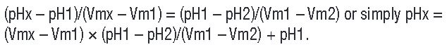
Several mathematical equations can be used to derive equation for the calibration. One of the commonly used formulas is a straight line equation using a point slope form. This equation uses two points taken during the calibration: P1 (Vm1, pH1) and P2 (Vm2, pH2), where P1 and P2 were the points taken using the chosen buffer soltions. To determine the pH level of the unknown solution, with a given point of Px (Vmx, pHx), a simple linear interpolation can be use with the equation:
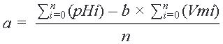
For a higher degree of accuracy given a multiple set of points, a first-order linear regression can be used. Given a set of n number of data points P0 (Vm0, pH0), P1 (Vm1, pH1), P2 (Vm2, pH2), P3 (Vm3, pH3), ... , Pn (Vmn, pHn), the general equation, pHx = a + b × Vmx, can be formulated using a least square method where b as the slope of the line and a is the intercept form having a value of:
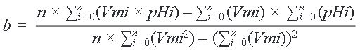
and
The least square method of approximation can be extended to the higher degree such as a second-order degree nonlinear equation. The general equation for the second order can be found as pHx = a + b × Vmx + c × Vmx2. Values for a, b, and c can be calculated as shown below:
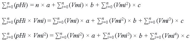
These systems of equations can be used to solve for the given unknown variables a, b, and c, through substitution, elimination, or through the matrix method.
Hardware Design Solutions
Buffer Amplifier
With this given condition, a buffer amplifier with high input impedance and very low input bias current is needed to isolate the circuit from this high source resistance. The AD8603 low noise op amp can be used as a buffer amplifier for this application. The low input current of the AD8603 minimizes the voltage error produced by the bias current flowing through the electrode resistance. For 200 fA typical input bias current, the offset error is 0.2 mV (0.0037 pH) for a pH probe that has 1 GΩ series resistance at 25°C. Even at the maximum input bias current of 1 pA, the error is only 1 mV. Though not necessary, guarding, shielding, high insulation resistance standoffs, and other such standard picoamp methods can be used to minimize leakage at the high impedance input of the chosen buffer.
Analog-to-Digital Converter
A low power ADC can be a favorable converter for this application. This is achievable using the AD7792, 16-bit Σ-Δ ADC for precision measurement applications. It has a 3-channel input that is low noise: only 40 nV rms noise when the update rate equals 4.17 Hz. The parts operate with a power supply from 2.7 V to 5.25 V, and it has a typical current consumption of 400 μA. The device is housed in a 16-lead TSSOP package. Added features include an internal band gap reference with 4 ppm/°C drift (typical), a 1 μA maximum power down current consumption, and an internal clock oscillator to reduce component count and PCB space.
Choosing the RF Transceiver
Based on the previous requirements, ADuCRF101 is the best fit for the intended application.
The ADuCRF101 is a fully integrated data acquisition solution designed for low power wireless applications. The ADuCRF101 operates at 431 MHz to 464 MHz and 862 MHz to 928 MHz. It is integrated with communication peripherals like the required two SPI buses. 128 kB of nonvolatile Flash/EE memory and 16 kB of SRAM are provided on chip. It is a one chip solution for microcontrollers and transceivers, thus minimizing the number of components and board size.
The ADuCRF101 operates directly from a battery with a supply range from 2.2 V to 3.3 V with power consumption of:
- 280 nA, in power-down mode, nonretained state
- 1.9 μA, in power-down mode, processor memory, and RF transceiver memory retained
- 210 μA/MHz, Cortex-M3 processor in active mode
- 12.8 mA RF transceiver in receive mode, Cortex-M3 processor in power-down mode
- 9 mA to 32 mA RF transceiver in transmit mode, Cortex-M3 processor
in power-down mode
Software Implementation
Software is a critical part of the wireless transmission system. It dictates how the system will behave and it also has an impact to the power consumption of the system. The system has two software parts—namely, the protocol stack and the application stack. The protocol stack used is the ADRadioNet, a wireless networking protocol for the ISM band. It uses IPv6 addresses and combines most of the features expected in such solutions—that is, low power, multihop, end-to-end acknowledgement, self-healing, and so on. The application stack is a software that accesses the pH reference design board via SPI.
To efficiently run the two software stacks, a simple scheduler was used. A nonpreemptive scheduler handles the protocol stack task; its functions are given a specific time and specific resources. However, the number of defined tasks in the system is limited. To operate efficiently, execution of the defined tasks must be completed by the nonpreemptive scheduler before its time lapses. With the two stacks in system, the nonpreemptive scheduler is a good fit because of the limited number of defined tasks assigned to it.
Conclusion
This article has presented different challenges and solutions for the design aspects of pH wireless sensor monitoring. It has been shown that ADI data acquisition products can essentially be used to address the given different challenges for pH measurement. The AD8603 op amp, or any equivalent ADI amplifier with high input impedance, can be used to counter the sensor’s high output impedance—therefore providing enough shielding to prevent system loading. The ADuCRF101 data acquisition system IC can provide a complete solution for RF data transmission. The accuracy of the data acquisition can be accomplished in hardware by using a precision amplifier and ADC, or it can also be accomplished by calibration in software using mathematical statistics to formulate a general equation such as different methods of curve fitting.
著者について


