Simplicity Wins—Part 4: The Algorithm Behind Efficient Active Balancing

×

Figure 1

   

Abstract

In general, the design of the active balancing algorithm varies depending on the hardware architecture it supports. Therefore, achieving a simplified balancing hardware design while also reducing the complexity of the algorithm design remains a key challenge that must be addressed. This article delves into the algorithm behind efficient active balancing design for battery management systems (BMS). It is important to note that, because balancing algorithms and hardware architectures is typically deeply integrated and co-optimized, the algorithm discussed here is primarily tailored to the architecture featured in this article series. Nevertheless, many of the design principles, trade-offs, and implementation ideas presented may serve as a source of inspiration for engineers developing balancing algorithms for other active balancing architectures.

Introduction

In the previous parts of this article series, the discussion mainly focused on how to select the right ICs and components to build an active balancing circuit or architecture. While balancing algorithms do play an important role in active balancing systems, they deserve further in-depth discussion.

Therefore, the objective of this article is to present an attempt at developing an algorithm specifically tailored for the balancing architecture featured in this series. The goal is to provide a reference design for an active balancing algorithm that is efficient, streamlined, and easy to deploy and evaluate—allowing engineers and practitioners to quickly implement, test, and directly observe the real-world balancing performance of ADI’s solution in battery packs.

That said, it is worth stressing—perhaps more than once—that despite the emphasis on the simplicity and efficiency of the proposed balancing algorithm, no single algorithm can seamlessly handle every possible cell mismatch scenario in practice. Any balancing strategy must be thoroughly evaluated and validated before deployment in a live battery system.

Active Balancing GUI Software

Building on the active balancing concepts introduced earlier in this series, the control code for the active balancing system is primarily deployed in two locations: the embedded microcontroller unit (MCU) and the PC-based active balancing GUI. While the role and functionality of the MCU have already been discussed in previous articles, this part focuses on the PC-side evaluation software—the active balancing GUI.

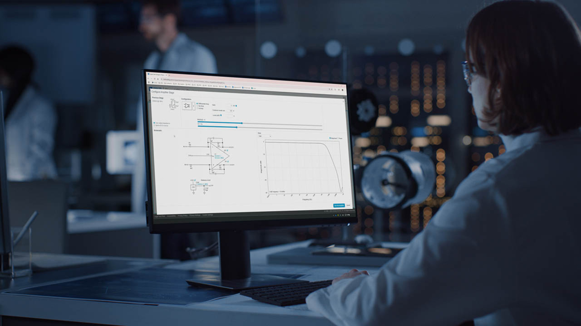
Figures 1 and 2 show screenshots of the GUI interface used in this design architecture. To avoid visual clutter, only features whose functions are not immediately obvious have been labeled for clarity.

The GUI serves as the communication bridge between the MCU and the computer, while also providing real-time data visualization. It displays cell voltages, indicates each cell’s balancing status, and captures as well as logs system faults or abnormal operating conditions. Most importantly, the GUI integrates an automated active balancing algorithm, making it not only a monitoring tool but also a key driver in executing the balancing process.

Performance Under Active Balancing Algorithm

This design architecture supports two modes of control for the active balancing process: manual balancing control and fully automated algorithm control.

1. Manual Balancing Control
   
   In manual mode, users can directly issue commands to charge, discharge, or disable balancing for an individual cell. This mode is useful for diagnostic testing or for performing targeted balancing interventions and fine-tuning specific cells.
2. Automated Active Balancing Algorithm
   
   In automated mode, the process is streamlined for ease of use: connect the battery pack to the system, launch the GUI software, establish serial communication with the MCU, and click the AUTO_ENABLE button. The system will then automatically bring all 16 cells to the same voltage level without further user intervention.

Figures 3 to 5 illustrate the convergence of cell voltages under three distinct operating conditions—charging, discharging, and idle—with the automated balancing function enabled. The battery pack used in testing consists of 16 NMC lithium-ion cells, each rated at 40 Ah.

• Charging state: The pack is charged using a 10 A maximum current charger. Cell voltages rise from roughly 3.65 V to near 4.1 V.
• Discharging state: The pack is connected to a 10 Ω high power resistive load, causing voltages to drop from around 3.85 V to approximately 3.65 V.
• Idle state: The pack is idle, with no charger or load connected.

In all three cases, the cell voltages were intentionally unbalanced at the start of the test to better demonstrate the convergence effect of the active balancing circuit. Once all cell deviations converged within the threshold—defined as within ±3 mV of the average voltage—the automatic balancing stop condition was triggered, and the experiment was terminated.

As shown in figures 3 to 5, enabling the automated algorithm results in the 16 cells converging to within a narrow voltage tolerance. This confirms that the proposed architecture and algorithm deliver consistent and effective balancing not only in idle conditions but also during both charging and discharging phases.

Execution Logic of the Automated Balancing Algorithm

The automated balancing algorithm operates in a cyclic, sequential manner—balancing each of the 16 cells in turn and then repeating the process. Instead of attempting to fully balance a single cell in one pass, it applies a round-robin strategy, performing multiple short balancing cycles. This avoids excessively long dwell times on individual cells, which could reduce the overall balancing throughput and potentially compromise pack safety. Extended focus on balancing a single cell can also introduce risks of overcharging or overdischarging other cells that are left idle for too long. By distributing balancing across all cells, deviations converge efficiently toward a predefined stop threshold.

The algorithm applies two complementary methods depending on cell grouping:

1. Buffer Balancing (Cells 2 to 9)—Relative Balancing
   
   • The average voltage of the buffer group (cells 2 to 9) is calculated and denoted as Avg(2 to 9).
   • Each buffer cell (cells 2 to 9) is balanced relative to Avg(2 to 9), rather than the overall pack average (AvgALL).
2. Independent Cell Balancing (Cell 1 and Cells 10 to 16)—Absolute Balancing
   
   • The overall pack average voltage across all 16 cells is calculated as AvgALL.
   • Each independent cell (cell 1 and cells 10 to 16) is balanced toward AvgALL.

For both buffer and independent cells, the balancing direction (charge or discharge) and balancing duration are determined by the sign and magnitude of each cell’s deviation. Although duration is roughly proportional to deviation, no single cell dominates the balancing process. The algorithm cycles through all cells in short, iterative passes, ensuring fast, stable convergence.

The ultimate goal of the balancing process is to bring all cells in the pack as close as possible to AvgALL. The reason for dividing the algorithm into “relative balancing” for the buffer group and “absolute balancing” for the independent cells is efficiency: if buffer cells were directly balanced against AvgALL, they would then still undergo repeated charge-discharge cycles while serving as an energy reservoir for the other cells. This would make convergence inefficient. By first aligning the buffer cells with Avg(2 to 9) through relative balancing, and then using the buffer as a whole to charge or discharge independent cells, the system achieves faster overall convergence. By the end of a complete balancing cycle, Avg(2 to 9) and AvgALL may not be perfectly identical, but they will be nearly equal, ensuring that the entire pack reaches a well-balanced state.

To further enhance efficiency and reliability, if a cell’s deviation is already within tolerance—or if an abnormal condition is detected—the algorithm skips that cell and continues to the next eligible one.

Architectural Rationale and Buffer-Based Balancing Mechanism

Attentive readers may notice that the balancing strategy described above differs from an ideal, fully bidirectional cell-to-cell balancing topology. The reason is straightforward: achieving true, direct bidirectional energy transfer between any two arbitrary cells within a pack is not practically feasible without introducing substantial architectural complexity.

To address this, the algorithm leverages an intermediate charge buffer to enable indirect balancing. Specifically, n adjacent cells within the pack are designated as the buffer—a configuration also reflected in Figure 6 of the balancing architecture diagram, where the buffer is depicted as a module composed of these n consecutive cells.

Unlike conventional designs that rely on independent external power sources to act as the buffer—such as large-capacity 12 V or 24 V batteries—this architecture operates entirely using energy already stored within the pack. This approach not only improves overall system efficiency but also reduces both hardware and software design complexity.

The balancing process in this architecture and algorithm is implemented via a two-step energy transfer.

1. Cell-to-Buffer Discharge: Energy from an overcharged cell is transferred into the buffer cells.
2. Buffer-to-Cell Recharge: Energy from the buffer is then redistributed to undercharged cells.

This two-stage sequence effectively achieves the functional equivalent of bidirectional cell-to-cell balancing, while avoiding the engineering complexity of implementing a direct, one-to-one transfer topology. Such a topology is considered the ideal form of balancing, but is often impractical to realize in large battery packs due to its circuit complexity and cost. In this approach, whenever a cell requires charging, the necessary energy is uniformly sourced from the buffer cells; conversely, when a cell needs to be discharged, its excess energy is evenly redistributed back into the buffer cells.

Conditions for Temporary Suspension and Reactivation of Automated Balancing

The automated balancing process temporarily suspends when the voltage deviation of cells 2 to 9 from Avg(2 to 9) falls below a defined threshold (for example, ±3 mV), and the deviation of cell 1 and cells 10 to 16 from AvgALL is also within the same threshold. At this point, Avg(2 to 9) and AvgALL may not be perfectly identical, but they will be nearly equal. Once these conditions are met, the algorithm transitions into a standby state, monitoring for the next balancing trigger.

When active, the automated balancing algorithm continuously polls the battery system to determine whether balancing is required. The trigger conditions are user-configurable; by default, balancing is initiated when the voltage spread—the difference between the highest and lowest cell voltages among the 16 cells—exceeds 10 mV.

Upon activation, the algorithm operates until the suspension criteria are reached, at which point it halts and waits for the next trigger event. As mentioned earlier, the suspension condition remains the same and will not be repeated here.

To prevent excessive cycling and unnecessary energy dissipation, a hysteresis band is applied between the trigger threshold (10 mV) and the suspension threshold (±3 mV). This ensures that balancing is only reactivated when a meaningful voltage deviation occurs, improving both efficiency and system longevity.

Special Considerations

Because the cell-voltage sampling harness and the active-balancing harness share the same wiring, and because of the presence of Rroute (as described earlier in this series) combined with the effect of large balancing currents, a voltage drop occurs during active balancing. This drop affects the accuracy of cellvoltage measurements, as illustrated in figures 7 to 10. Therefore, active balancing must be periodically paused to obtain accurate voltage readings.

• If pauses occur too frequently, balancing efficiency is reduced.
• If pauses occur too infrequently, overbalancing may occur.

In this architecture, the algorithm estimates the required balancing duration based on the observed voltage deviation—for example, every 5 mV of deviation corresponds to approximately 1 minute of balancing. After this calculated duration, balancing is auto paused to take accurate voltage measurements, and the algorithm then decides the next course of action.

This adaptive timing strategy improves efficiency compared to fixed-interval methods, but it relies on the assumption of a nearly constant charging/discharging current. In this design, the current stability is achieved by sourcing the buffer voltage directly from the battery pack itself rather than from an external power supply, ensuring nearly constant current flow even as cell voltages vary from 3.0 V to 4.2 V.

Although combining the sampling harness and balancing harness introduces measurement errors during balancing, it also provides notable benefits:

• It reduces the number of harnesses, simplifies wiring, and saves PCB space.
• The voltage drop observed during balancing can serve as an operational indicator, helping to confirm whether the active balancing circuit is functioning properly.

Conclusion

With this, the entire series on active balancing comes to a close. Naturally, detailing every aspect of such a systematic design within a limited space is challenging, even with extensive explanations. Many intricate design elements—particularly the comprehensive software programming involved in this active balancing solution—cannot be fully covered here.

The primary goal of this series is to spark curiosity and inspire engineers and electronics enthusiasts interested in active battery balancing. Readers are encouraged to either adopt the design presented or build upon it, continuously innovating to develop active balancing solutions that embody simplicity and efficiency.

About the Authors