AN-2585: GMSL3 Channel Specification
Abstract
The GMSL3 Channel Specification defines the hardware system design requirements necessary for proper operation of GMSL3 devices. It should be used in conjunction with the relevant GMSL3 serializer and deserializer data sheets to develop compliant GMSL3 systems.
Purpose and Scope
The GMSL3 Channel Specification defines the hardware system design requirements necessary for proper operation of GMSL3 systems as specified by device datasheets. It contains both the GMSL3 System Channel Specification and the GMSL3 Module Channel Specifications. Within this document, “GMSL3 Channel Specification” is used to collectively refer to the specifications.
This document describes important system design considerations and should be used as a reference for system development and component evaluation. Relevant system elements include PCB material, PCB layout, passive PCB components, cable(s), and connectors.
Compliant GMSL3 systems meet or exceed the S-parameter curves, crosstalk specifications, and link margin requirements detailed in this document.
A compliant GMSL3 system channel has an expected bit error ratio (BER) of 10-30 or better when FEC is used.
GMSL3 Channel Descriptions and Definitions
GMSL3 Overview
GMSL3 devices use ADI’s proprietary third-generation gigabit multimedia serial link (GMSL3) technology to transport high-speed serialized data over coax or shielded twisted-pair cable for automotive camera and display applications.
GMSL3 devices use a pulse amplitude modulation – 4 Level (PAM4) encoding scheme to allow links to operate at a fixed data rate of 12Gbps on the forward channel, the reverse channel operates at 187.5Mbps.
PAM4 is an encoding scheme that uses 4 discrete voltage levels. This differs from the encoding scheme used for GMSL2 devices, which uses non-return-zero (NRZ) encoding. PAM4 has 2bits per symbol whereas NRZ is only 1bit per symbol, which is why GMSL3 has double the data rate with the same symbol rate. The PAM-4 eye height is reduced by 8dB when compared to a NRZ eye. GMSL3’s 12Gbps PAM4 link utilizes Forward Error Correction (FEC) to increase robustness of the link on very long channels.
NRZ vs. PAM4 Encoding Scheme differences is shown below in Figure 1.

Figure 1. NRZ vs. PAM4 Encoding Temporal Characteristics.
A block diagram of a typical GMSL3 system is shown below in Figure 2.

Figure 2. GMSL3 System Block Diagram.
*Note: The forward channel is defined as serializer-to-deserializer transmission; the reverse channel is defined as deserializer-to-serializer transmission.
GMSL3 Channel Definition

Figure 3. GMSL3 Channel Definition.
Note: AC-coupling capacitors and optional power over coax (PoC) or line-fault components are not depicted in Figure 3.
The GMSL3 Module Channels is defined as the Pin-to-Pin Channel from the SIO pin(s) of the serializer to the SIO pin(s) of the deserializer and consists of the following:
- Serializer PCB Channel
- Cable Channel
- Deserializer PCB Channel
Note: For multi-link configurations (i.e., dual link, splitter mode, and reverse splitter mode) each GMSL link is treated as an independent Pin-to-Pin Channel.
The GMSL3 Module Channels are defined as the individual sub-channels within the GMSL3 System Channel.
The PCB Channel is defined as the channel from the device SIO pin to the end of the PCB-mounted connector. It includes the trace itself and any PCB components on the trace (e.g., line-fault resistors, PoC components, ESD diodes, common mode chokes, and other passive components). This channel is also referred to as the Serializer or Deserializer PCB Channel Module and can be evaluated for GMSL3 Module Compliance.
The Cable Channel is defined inclusively as the channel comprising all components from the cable connector on the serializer side to the cable connector on the deserializer side, including the cable(s) and any in-line connector(s). For applications using cable bundles, the cable crosstalk specification must consider the other conductors in the cable harness. This channel is also referred to as the Cable Module and can be evaluated for GMSL3 Module Compliance.
Note: Meeting module compliance requirements guarantees GMSL3 System Channel Compliance when implemented with other compliant modules and cable(s).
GMSL3 Channel Frequency Bands
GMSL3 is a packet-based protocol operating at a fixed link-rate. The GMSL3 forward channel data rate is 12Gbps, the reverse channel data rate is 187.5Mbps. The transmitted/received data rate is a fixed rate based on the data rate setting and is independent of the payload. For example, if a camera or display application requires 10Gbps, the forward channel data rate on the link must be set to 12Gbps and idle data will fill the unused link capacity.
Forward Channel:
The GMSL3 forward channel uses PAM4 encoding scheme and transfers 2bits per symbol. A key frequency
for PAM4 encoding is ¼ bit rate, for a 12Gbps PAM4 channel (GMSL3 Forward Channel) it is 3GHz.
Reverse Channel:
The GMSL3 reverse channel uses a non-return to zero (NRZ) encoding scheme. A key frequency of NRZ
encoding is ½ bit rate, for a 187.5Mbps NRZ channel (GMSL3 Reverse Channel) it is 93.75MHz.
Note: that the maximum frequency defined in the channel specification is higher than the key frequencies listed above. This is due to the energy content of the rise/fall times of the transmitters. The attenuation (due to insertion loss) of the signal at the key frequencies is the most critical value to consider when exploring the maximum channel length that can be used in a system. However, the specification must be met across the entire frequency band defined.
| GMSL – Speed | Minimum Frequency | Key Frequency | Maximum Frequency specified in Channel Specification |
| Forward Channel – 12Gbps | 2MHz | 3GHz | 3.5GHz |
| Reverse Channel – 187.5Mbps | 2MHz | 93.75MHz | 3.5GHz |
Note: The crosstalk specifications extend across a greater frequency band than the return loss and insertion loss specifications.
The bidirectional transmitter/receiver of GMSL3 necessitates emphasis on return loss. The energy of the forward and reverse channels overlap in frequency, so reflections in the band of the low-speed transmitter and receiver are especially important to consider when designing the channel. For system optimization, insertion loss must be minimized and return loss must be optimized.
Network Analyzer Settings:
The recommended settings for data capture are 100kHz to 4GHz with 1MHz or smaller step size. The frequency
steps should be linear and not logarithmically spaced.
GMSL3 Channel S-parameter Definitions
The GMSL3 Channel Specification defines minimum or maximum values of scattering parameters (S-parameters) across the frequency band of interest in a 50Ω environment. S-parameters are defined for insertion loss and return loss. Reference Figure 4 and the corresponding sections below. For the GMSL3 Channel Specification, the serializer is defined as Port 1 and the deserializer is defined as Port 2.

Figure 4. GMSL3 Channel S-Parameter Definitions.
Insertion Loss (S21/Sdd21, S12/Sdd12)
Insertion loss is the energy loss across the transmission channel.
- S21/Sdd21 – Forward channel insertion loss
- S12/Sdd12 – Reverse channel insertion loss
S21/Sdd21 defines the amount of energy loss for the high-speed channel (forward channel), and S12/Sdd12 defines the amount of energy loss for the low-speed channel (reverse channel). For typical GMSL3 channels consisting of passive PCB components and cables, S21/Sdd21 and S12/Sdd12 are equal.
For differential applications (i.e., STP), use differential S-parameters (Sdd21 and Sdd12). For more information regarding S-parameter definitions, see Appendix A: Single-Ended and Differential S-parameters.
Return Loss (S11/Sdd11, S22/Sdd22)
Return loss is the reflected energy back to the transmitter.
- S11/Sdd11 – Forward channel return loss
- S22/Sdd22 – Reverse channel return loss
S11/Sdd11 is used to evaluate the high-speed transmitter energy reflected into the low-speed receiver; S22/Sdd22 is used to evaluate the reflected energy of the low-speed transmitter back into the high-speed receiver.
For differential applications (i.e., STP), use differential S-parameters (Sdd11 and Sdd22). For more information regarding S-parameter definitions, see Appendix A: Single-Ended and Differential S-parameters
GMSL3 System Channel Specification

Figure 5. GMSL3 System Channel.
GMSL3 System Channel Compliance
A compliant GMSL3 system must meet the overall Pin-to-Pin Channel Specification, including the S-parameter curves, crosstalk specification, and the link margin requirements under worst-case conditions* as defined by the system designer.
A short channel limit allows low-loss links to have increased return loss. Low insertion-loss links have a large FWD channel amplitude allowing the return loss limit to be relaxed.
*Worst-case conditions include longest cable (highest insertion loss), cable aging effects, channel degradation due to temperature, PCB impedance variation, min/max system PoC loads. Worst-case conditions can be simulated; contact cable manufacturer and PCB designer for technical advice.
Note: The PCB and Cable Channels comprising a compliant GMSL3 System Channel may not meet the standards required for GMSL3 Module Compliance. Modules must be independently evaluated for Module Compliance. See the GMSL3 Module Channel Specifications section for additional information.
Filtering S-parameter Data
The S-parameter data must be filtered before comparing it to the GMSL3 Insertion Loss and Return Loss limits. A 100MHz wide filter is applied to the data across the full range. Unfiltered data should be used from the lowest frequency captured up to 50MHz. Beyond 50MHz the filtered data should be used to compare against the limits. Data capture should be set to linear frequency spacing so that filtering of data is simpler.
The filtering is accomplished by running a 100MHz wide moving average of the S-parameter data once converted to linear power amplitude. After the averaging has been accomplished the data is converted back to power in decibels for plotting against the limits.
Below are equations for converting S-parameters to linear power and back to dB power.

Equation 1. Conversion of real-imaginary S-parameters to linear power

Equation 2. Conversion of dB power S-parameters to linear power

Equation 3. Conversion of linear power S-parameters to dB power
Examples of filtering s-parameters are in Appendix B: Examples of Filtered S-parameters using MATLAB
GMSL3 Pin-to-pin Channel Specification
Maximum Insertion Loss Specifications (Pin-to-Pin)
- Defined by filtered S21 and S12 (or Sdd21 and Sdd12 for differential channels)
- Separate short and long channel limits
| Channel | Maximum Insertion Loss at Nyquist Frequency |
| Short (low loss) | –10dB @ 3GHz |
| Long (high loss) | –18dB @ 3GHz |

Figure 6. Pin-to-Pin Maximum Insertion Loss.
Short channel: links that have loss falling within the “short channel” insertion loss limit only need to meet the “short channel” return loss limit which is more lenient. The equations provided below can be used to calculate and plot insertion loss profiles of each forward/reverse channel configuration.
| Channel | Measurement Frequency Range [MHz] | Insertion Loss [dB] (f = Frequency [Hz]) |
| Short (low loss) | 2–3500 |  |
| Long (high loss) | 2–3500 |  |
Refer to Appendix B: Examples of Filtered S-parameters using MATLAB.
Maximum Return Loss Specification (Pin-to-Pin Channel)
- Defined by filtered S11 and S22 (or Sdd11 and Sdd22 for differential channels)
- Separated into short-channel and long-channel limits
- Short channels have a relaxed return loss limit above 800MHz

Figure 7. Pin-to-Pin Max Return Loss (Low Frequency).

Figure 8. Pin-to-Pin Max Return Loss.
The equations provided below can be used to calculate and plot return loss profiles of each forward/reverse channel configuration.
| Channel | Measurement Frequency Range [MHz] | Insertion Loss [dB] (f = Frequency [Hz]) |
| Short (low loss) | 2–10 | – 9– 0.9(𝑓 × 10–6) |
| 10–800 | –18 | |
| 800–3000 | – 16.9+ 8(𝑓 × 10–9– 1)/1.5 | |
| 3000–3500 | –6.2 | |
| Long (high loss) | 2–10 | – 9– 0.9(𝑓 × 10–6) |
| 10–1000 | –18 | |
| 1000–2500 | – 23.33 + 5.33(𝑓 × 10–9) | |
| 2500 | –10 |
Refer to Appendix B: Examples of Filtered S-parameters using MATLAB.
GMSL3 Crosstalk Specification
The GMSL3 crosstalk specification places limits on the permissible parasitic coupling from GMSL3, other high-speed links “aggressors” , and/or noise sources onto a GMSL3 link. Separate specification items for the PCB Module at the end of a link and the cable bundle allow system components to be individually developed and evaluated for crosstalk.
Crosstalk Specification for the PCB Module
Crosstalk between multiple ports on a PCB (e.g., an ECU) can be characterized in different ways depending on the source of the crosstalk and whether the interfering signals are narrowband or broadband in nature.
Crosstalk from GMSL or Other Broadband Signals
The setup shown in Figure 9 is used to measure crosstalk between the different ports (connectors) on a PCB. The data traffic causing interference is running on Ports 1..N, and crosstalk is measured on Port M of the PCB. The worst-case crosstalk condition occurs with cables with minimum insertion loss. This maximizes the received signal power on Port M. Crosstalk is measured as peak amplitude on Port M using an oscilloscope. Broadband crosstalk limits are presented in Table 5.
| Forward Data Rate [Gbps] | Reverse Data Rate [Mbps] | Measurement Frequency Range [MHz] | Maximum Crosstalk | Conditions |
| 12 | 187.5 | 1-4000 | <3mV(p-p) | Interferers are any combination of high-speed links |
In Figure 9, links from Devices 1..N are active. Crosstalk is measured on Port M with Device M in squelch mode.

Figure 9. Broadband Crosstalk Characterization Method.
Crosstalk from Narrowband Signals
If the interfering signal is a continuous wave or narrowband signal (e.g., a clock or switching frequency from a voltage regulator or a PoC circuit), the crosstalk into the GMSL port is measured in mV as shown in Figure 10 If the measured signal is a continuous wave, an oscilloscope or a spectrum analyzer can be used to measure the crosstalk voltage on the disturbed port (convert from dBm to mV). If the interfering signal is a complex waveform (e.g., a modulated waveform), an oscilloscope should be used. A low-noise amplifier and a bandpass filter may be required to obtain a clean measurement.
The limits in Table 6 are frequency-dependent because the GMSL receiver input amplifier adaptively compensates for the frequency-dependent loss of the cable by boosting high-frequency gain. The higher the frequency-dependent attenuation of the cable, the more the high-frequency portion of the received signal will be boosted by the serial link receiver. An unwanted side effect of this high-frequency boost is increased sensitivity to high-frequency crosstalk.
| Device | Forward/Reverse Data Rate | Measurement Frequency Range [MHz] | Peak-to-Peak Voltage Limit [mV](f = Frequency [MHz]) |
| Serializer | 12Gbps/187.5Mbps | 0.1–2 | 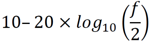 |
| 2–4500 | 10 | ||
| 4500–10000 | 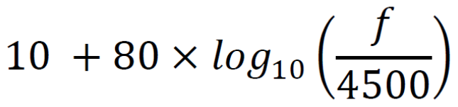 |
||
| Deserializer | 12Gbps/187.5Mbps | 0.1–2 | 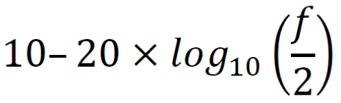 |
| 2–50 | 10 | ||
| 50–4500 | 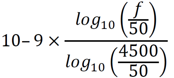 |
||
| 4500–10000 | 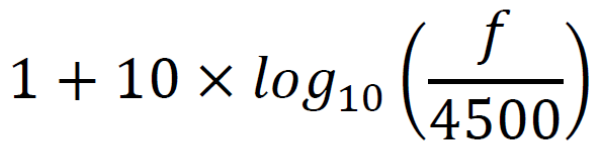 |
*Note: These limits include ripple injected by the PoC circuit.

Figure 10. Measurement Setup for Narrowband Crosstalk.


Figure 11. Narrowband Crosstalk Limits.
Crosstalk Specification for the Cable Bundle
Crosstalk occurs when multiple cables are routed together in a harness. ADI specifies both near-end crosstalk (NEXT) and far-end crosstalk (FEXT) for the case that multiple GMSL3 links are routed in the same harness.
| Data Rate | Noise source → GMSL Device | Frequency Range [MHz] | Specification Limit |
| 12Gbps forward, 187.5Mbps reverse | Serializer → Serializer | 1–4000 | NEXT < -35dB PS_ACR_F < -45dB |
| 12Gbps forward, 187.5Mbps reverse | Deserializer → Serializer Serializer → Deserializer Deserializer → Deserializer |
1–4000 | NEXT < -45dB PS_ACR_F < -45dB |
*Note: The metric for FEXT is Power-Sum Adjusted Crosstalk Ratio – Far End (PS_ACR_F).
See Far-End Cable Bundle Crosstalk for additional information.
Near-End Cable Bundle Crosstalk

Figure 12. Near-End Crosstalk (NEXT).
The near-end crosstalk is usually dominant. NEXT is based on the injection and measurement ports shown in Figure 12 and is specified as the power sum of the coupling from Ports 1..N into Port M (Equation 4).

Equation 4. Near End Crosstalk Equation
The NEXT measurement is performed as a sequence of multi-port S-parameter measurements using a vector network analyzer (VNA). The transfer functions from injection port to measurement port are added in the power domain.
*Note: During measurement, all unused ports must be terminated in 50Ω for coax or 100Ω for STP.
As an example, assume two interferers with transfer functions SM1 = −60dB and SM2 = −66dB. The power sum of SM1 and SM2 is found by converting both parameters from dB to power and converting the sum of power back to dB. NEXT is calculated as:

The resulting NEXT = -59dB, which satisfies the requirement for NEXT in Table 7.
Far-End Cable Bundle Crosstalk

Figure 13. Far-End Crosstalk (FEXT)
Far-end crosstalk (FEXT) is a measure of the crosstalk received at the far end of the cable with the disturbance applied at the near-end of the cable (Figure 13). The metric for FEXT is Power-Sum Adjusted Crosstalk Ratio – Far End (PS_ACR_F). The received amplitude on the measurement Port M of each interferer is attenuated by the transfer function SMi. Similarly, the wanted signal received at Port M will be attenuated by the insertion loss SMP of the disturbed cable. Assuming that the transmitted amplitude of all the interfering signals is the same, the far-end crosstalk measure, PS_ACR_F, represents the ratio of the interferers to the received wanted signal, providing a measure of interference-to-signal ratio in the disturbed cable. In the dB domain, this becomes a simple subtraction (Equation 5).

Equation 5. Power-Sum Adjusted Crosstalk Ratio – Far-End Crosstalk Equation
The PS_ACR_F measurement is performed as a sequence of two-port measurements using a VNA, and the results are added in the power domain as shown in Equation 5.
*Note: During measurement, all unused ports must be terminated in 50Ω for coax or 100Ω for STP.
As an example, assume two interferers with transfer functions SM1 = −70dB and SM2 = −70dB. SMP = −11dB. The power sum (calculated in the same manner as NEXT above) of SM1 and SM2 is −67dB. The resulting far-end crosstalk is PS_ACR_F = −67dB –− (−11dB) = −56dB, which meets the requirement for FEXT in Table 7.
GMSL3 Link Margin Specification
Link margin is specifically used to quantitatively test the signal integrity of the GMSL link.
The link margin test starts at the default transmit voltage amplitude for both the forward and reverse channels.
Forward Channel:
The test decreases the forward transmit amplitude in 10mV steps and monitors the Forward Error Correction
block input Bit Error Ratio (Link error ratio before FEC). The test stops when the FEC block input BER is > 1e-7 or there are un-corrected FEC blocks. The link margin is reported as the difference between the default
transmitter amplitude and when the link margin test stops.
Reverse Channel:
The test decreases the transmit amplitude in 10mV steps and performs an error check before proceeding to
the next test amplitude. The test ends at any point an error is detected. The link margin is reported as the
difference between the default transmitter amplitude and the amplitude at which the error was detected.
Table 8 below contains the required minimum link margin for both the forward and reverse channels.
| Cable | Data Rate (Forward/Reverse) | Minimum Required Forward Channel Link Margin [mV] | Minimum Required Reverse Link Margin [mV] |
| COAX/STP | 12Gbps/187.5Mbps | 100 | 50 |
*Note: A link margin tool is available through the ADI GMSL GUI. Alternatively, software support is available for customers who wish to develop their own implementation of these tools in their software.
GMSL3 Module Channel Specifications

Figure 14. GMSL3 Module Channels.
GMSL3 Module Compliance
Meeting module compliance requirements assists in meeting GMSL3 System Channel Compliance when implemented with other compliant modules and cable(s).
For GMSL3 Module Compliance:
- Serializer/Deserializer Module Channels must meet the PCB insertion loss and return loss requirements under worst-case conditions* as defined by the system designer.
- Cable Module Channels must meet the cable insertion loss and return loss requirements under worst-case conditions* as defined by the system designer.
* Worst-case conditions include longest cable (highest insertion loss), cable aging effects, channel degradation due to temperature, PCB impedance variation, min/max system PoC loads. Worst-case conditions can be simulated; contact cable manufacturer and PCB designer for technical advice.
*Note: A module meeting the GMSL3 Module Compliance Specification is interoperable with other compliant modules.
*Note: The PCB and Cable Channels comprising a compliant GMSL3 System Channel may not meet the standards required for GMSL3 Module Compliance. Modules must be independently evaluated for GMSL3 Module Compliance.
Maximum Insertion Loss Specification (PCB & Cable Modules)
- Defined by filtered S21 and S12 (or Sdd21 and Sdd12 for differential channels)
- Separate short and long channel limits for cable modules
| GMSL – Speed | Minimum Frequency | f½Linkrate |
| Cable | Short (low loss) | –7.6dB @ 3GHz |
| Long (high loss) | –15.6dB @ 3GHz | |
| PCB | Short & Long | –1.2dB @ 3GHz |

Figure 15. Maximum Cable Insertion Loss.

Figure 16. Maximum PCB Insertion Loss.
The equations provided below can be used to calculate and plot insertion loss profiles for both PCB and Cable system segments of each forward/reverse channel configuration.
| Module | Channel | Measurement Frequency Range [MHz] | Insertion Loss [dB] (f = Frequency [Hz]) |
| PCB | Low Loss and High Loss | 2–500 | – 0.5 |
| 500–3500 | – (0.36 + 0.28(𝑓 × 10–9)) | ||
| Cable | Short (Low Loss) | 2–3500 | 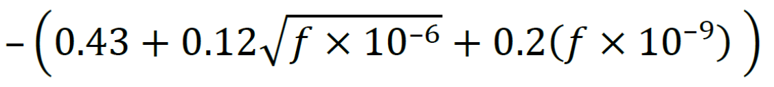 |
| Long (High Loss) | 2–3500 |  |
Maximum Return Loss Specification (PCB & Cable Modules)
- Defined by filtered S11 and S22 (or Sdd11 and Sdd22 for differential channels)
- Separate short and long channels limits
- Short channels have a relaxed return loss limit above 800MHz

Figure 17. Maximum Return Loss (PCB & Cable, low freq.).

Figure 18. Maximum Return Loss (PCB & Cable).
*Note: Return loss is not additive. Thus, there is not an “allowable” dB value of return loss for each section of the GMSL3 link (i.e., PCBs and Cable); the full link (i.e., pin-to-pin) must meet the pin-to-pin specified return loss allocation. For links that achieve the short-channel insertion loss specification, the relaxed return loss specification (short channel) applies.
*Between the frequency range of 2-10MHz, PCB and Cable channels have a different return loss specification to allow for power-over-coax (PoC) networks on the PCBs. Do not use filtered data below 10MHz. Reference equations below for more information.
The equations provided below can be used to calculate and plot return loss profiles for both PCB and Cable system segments of each forward/reverse channel configuration.
| Module | Channel | Measurement Frequency Range [MHz] | Insertion Loss [dB] (f = Frequency [Hz]) |
| PCB | Short (low loss) | 2–10 | – 9– 0.9(𝑓 × 10–6) |
| 10–800 | –18 | ||
| 800–3000 | – 16.9 + 8(𝑓 × 10–9–1)/1.5 | ||
| 3000–3500 | –6.2 | ||
| Long (high loss) | 2–10 | –9 – 0.9(𝑓 × 10–6) | |
| 10–1000 | –18 | ||
| 1000-2500 | – 23.33 + 5.33(𝑓 × 10–9) | ||
| 2500–3500 | –10 | ||
| Cable | Short and Long | 2–1000 | –18 |
| 1000–2500 | – 23.33 + 5.33(𝑓 × 10–9) | ||
| 2500–3500 | –10 |
Appendix A: Single-ended and Differential S-parameters
S-parameters (scattering parameters or scattering matrix) are used to characterize the ADI GMSL3 channel specification requirement. S-parameters are used to quantify how RF energy propagates through a multi-port network. For COAX mode, which uses single-ended signaling, the channel is characterized as a two-port, single-ended network (Figure 19). These networks have one input port and one output port. Signals on the input and output ports are referenced to ground. Measurements should be made using a vector network analyzer.
*Note: The GMSL3 Channel Specification applies to the componentry and cabling from the pin(s) of the transmitter to the pin(s) of the receiver. See GMSL3 Channel Definition above for additional information.

Figure 19. Two-Port, Single-Ended Network.
STP mode requires the use of differential S-parameters (Sdd) to evaluate the network. Differential S-parameters can be taken as single-ended, four-port measurements and converted to differential parameters using matrix math. For measurement purposes, the two-port differential network (Figure 20) can be considered a four-port, single-ended network (Figure 21).

Figure 20. Two-Port, Differential Network.

Figure 21. Four-Port, Single-Ended Network.
*Note: Mixed-mode S-parameters can be extracted from S4P files (or four-port, single-ended S-matrix) with the standard formula or professional tools. Some network analyzers will output differential S-parameters directly when set up to do so.
Appendix B: Examples of Filtered S-parameters Using MATLAB
The return loss data must be filtered before comparing it to the GMSL3 return loss limit. A 100MHz filter is applied to the S-parameters across the full range. Unfiltered data should be used from the lowest frequency captured up to 50MHz. Beyond 50MHz the filtered data should be used to compare to the limit. Data capture should be set to linear frequency so that filtering of data is simpler.
Single Ended S-parameters
The following is an example of MATLAB code used to filter S-parameter data and plots showing difference between unfiltered and filtered data. The S-parameter data is in real-imaginary format and is of a s2p file. The function includes the GMSL3 pin-to-pin limits.
    function [freq, Sxy_dB, Sxy_filt_dB, RL_lim_short, RL_lim_long, IL_lim_short, IL_lim_long] = filterSxy(x)
        Sxy = sparameters(x);
        freq = (Sxy.Frequencies);
        f_window = 100*10^6;
        points = numel(freq);
        f_step_size = (max(Sxy.Frequencies)-min(Sxy.Frequencies))/(points - 1);
        w_size = round(f_window/f_step_size);
        Sxy_array = [rfparam(Sxy,1,1) rfparam(Sxy,1,2) rfparam(Sxy,2,1) rfparam(Sxy,2,2)];
        Sxy_V_mag = abs(Sxy_array);
        Sxy_Power_mag = Sxy_V_mag.^2;
        Sxy_dB = 10*log10(Sxy_Power_mag);
        Sxy_filt = smoothdata(Sxy_Power_mag,"movmean",w_size);
        Sxy_filt_dB = 10*log10(Sxy_filt);
        RL_lim_short = [0.002 -10.8; 0.01 -18; 0.8 -18; 3 -6.2; 3.5 -6.2];
        RL_lim_long = [0.002 -10.8; .01 -18; 1 -18; 2.5 -10; 3.5 -10];
        IL_range_GHz = transpose(0.01 : 0.01 : 3.5);
        IL_lim_short = [IL_range_GHz -(1.45+0.101*sqrt(IL_range_GHz*1000)+1.01*IL_range_GHz)];
        IL_lim_long = [IL_range_GHz -(1.62+0.182*sqrt(IL_range_GHz*1000)+2.14*IL_range_GHz)];
   end
The function can be saved in a MATLAB workspace and a set of S-parameters can be filtered and plotted by typing the following commands:
    [freq, Sxy_dB, Sxy_filt_dB, RL_lim_short, RL_lim_long, IL_lim_short, IL_lim_long] = filterSxy
    ('filename.s2p');
    plot(freq/10^9, Sxy_filt_dB);
    xlim([0 4]);
    hold on;
    plot(RL_lim_short(:,1), RL_lim_short(:,2));
    plot(RL_lim_long(:,1), RL_lim_long(:,2));
    plot(IL_lim_short(:,1), IL_lim_short(:,2));
    plot(IL_lim_long(:,1), IL_lim_long(:,2));
    ylabel('Sxy [dB]');
    xlabel('Frequency [GHz]');
    legend('S11','S12','S21','S22','RL Limit Short', 'RL Limit Long', 'IL Limit Short', 'IL Limit
    Long');
To plot the unfiltered data use the command: plot(freq/10^9, Sxy_dB);
Differential S-parameters
The following example shows the MATLAB code to take single-ended, 4-port measurements of a differential channel and convert it to differential S-parameters (Sdd11, Sdd12, Sdd21, Sdd22) and filter the results for comparison to the pin-to-pin GMSL3 channel specifications.
    function [freq, Sxy_dB, Sxy_filt_dB, RL_lim_short, RL_lim_long, IL_lim_short, IL_lim_long] = filterSxydiff(x)
        Sxy = sparameters(x);
        freq = (Sxy.Frequencies);
        f_window = 100*10^6;
        points = numel(freq);
        f_step_size = (max(Sxy.Frequencies)-min(Sxy.Frequencies))/(points - 1);
        w_size = round(f_window/f_step_size);
        S1 = Sxy.Parameters;
        S2 = s2sdd(S1);
        S3 = [S2(1,1,:) S2(1,2,:) S2(2,1,:) S2(2,2,:)];
        S4 = squeeze(S3);
        S5 = transpose(S4);
        Sxy_Vmag = abs(S5);
        Sxy_Power_mag = Sxy_Vmag.^2;
        Sxy_dB = 10*log10(Sxy_Power_mag);
        Sxy_filt = smoothdata(Sxy_Power_mag,"movmean",w_size);
        Sxy_filt_dB = 10*log10(Sxy_filt);
        RL_lim_short = [0.002 -10.8; 0.01 -18; 0.8 -18; 3 -6.2; 3.5 -6.2];
        RL_lim_long = [0.002 -10.8; .01 -18; 1 -18; 2.5 -10; 3.5 -10];
        IL_range_GHz = transpose(0.01 : 0.01 : 3.5);
        IL_lim_short = [IL_range_GHz -(1.45+0.101*sqrt(IL_range_GHz*1000)+1.01*IL_range_GHz)];
        IL_lim_long = [IL_range_GHz -(1.62+0.182*sqrt(IL_range_GHz*1000)+2.14*IL_range_GHz)];
   end
The function can be saved in a MATLAB workspace and a set of S-parameters can be filtered and plotted by typing the following commands:
    [freq, Sxy_dB, Sxy_filt_dB, RL_lim_short, RL_lim_long, IL_lim_short, IL_lim_long] = filterSxydiff
    ('filename.s4p');
    plot(freq/10^9, Sxy_filt_dB);
    xlim([0 4]);
    ylim([-35 0]);
    hold on;
    plot(RL_lim_short(:,1), RL_lim_short(:,2));
    plot(RL_lim_long(:,1), RL_lim_long(:,2));
    plot(IL_lim_short(:,1), IL_lim_short(:,2));
    plot(IL_lim_long(:,1), IL_lim_long(:,2));
    ylabel('Sxy [dB]');
    xlabel('Frequency [GHz]');
    legend('Sdd11','Sdd12','Sdd21','Sdd22','RL Limit Short', 'RL Limit Long', 'IL Limit Short', 'IL
    Limit Long');
To plot the unfiltered data use the command: plot(freq/10^9, Sxy_dB);
Example of a Passing Channel
The example below is of three series 0.5m coaxial cables and includes the replica traces of the IC to cable connectors on each end of the link such that it represents the pin-to-pin S-parameters of the GMSL3 channel.

Figure 22. Pin-to-Pin Insertion Loss vs. Limit.

Figure 23. Pin-to-Pin Return Loss vs. Limit.
The combination of the PCBs plus three series 0.5m cables creates significant reflected energy, but the insertion loss is low and falls within the “short channel” category, hence the filtered S11 passes the short channel return loss limit. Note that analysis must be completed for S12 and S22 as well.
RESULTS: Passes GMSL3 insertion loss and return loss limits.
Example of a Failing Channel
The example below is of a 5m STP cable and includes the replica traces of the IC to cable connectors on each end of the link such that it represents the pin-to-pin S-parameters of the GMSL3 channel.

Figure 24. Pin-to-Pin Insertion Loss vs. Limit.

Figure 25. Pin-to-Pin Return Loss vs. Limit.
In this example, the differential data from MATLAB was plotted in Excel. The poor layout of the PCBs creates significant reflected energy. The filtered insertion loss falls within the long channel limit and the return loss is compared to the long channel return loss limit. The filtered S11 fails the long channel return loss limit.
RESULTS: Fails GMSL3 return loss limit.
Example of a Channel with Power-Over-Coax (PoC)
The following example is for a coaxial link that includes three series cables (10m + 3m + 0.5m) along with a PoC network on the PCBs operating with 600mA current.

Figure 26. Pin-to-Pin Insertion Loss vs. Limit.

Figure 27. Pin-to-Pin Return Loss vs. Limit (low frequency).

Figure 28. Pin-to-Pin Return Loss vs. Limit.
RESULTS: Passes GMSL3 insertion loss and return loss limits.