×

Figure 1

   

摘要

Within the appliance motor control industry there is an increasing trend to move towards using brushless dc motors. This trend is in response to recent legislation mandating improved efficiency standards in appliance applications. Brushless dc motors do however require rotor position information in order to select the appropriate commutation angle. In cost sensitive applications such as appliances a sensorless commutation scheme is often desirable. This paper describes the development of such an algorithm based on an Extended Kalman estimator. In its simplest form this algorithm provides estimates for position and velocity based on the back-EMF segments from a trapezoidal driven motor. Unlike previous sensorless algorithms, based on the Extended Kalman techniques, this algorithm doesn’t require stator current measurements. The algorithm simply requires four resistor divider networks to scale the three back-EMF and dc link voltages and a low cost embedded DSP motor controller.

Introduction

Recent legislation imposing efficiency standards in appliances has forced appliance manufacturers to migrate to brushless dc motors in their applications. The introduction of brushless dc motors has however increased the level of complexity in controlling these applications. Moreover, brushless dc motors typically require some form of position transducer in order to select the correct commutation sequence. However in such cost sensitive applications the additional cost associated with adding position transducers is not acceptable or even practical. The traditional sensors were Hall sensors mounted in the machine. This requires more complex machine construction and can reduce the reliability of the overall system. This paper presents a sensorless control algorithm for a brushless dc motor, which requires only four resistor divider networks from which estimates of position, velocity, and disturbance torque information can be derived. Furthermore this algorithm provides instantaneous position and velocity information unlike the classical zero crossing approach.

This algorithm was developed for and implemented on the Analog Devices ADMC330 DSP motor controller [Murray 96]. The algorithm requires approximately 500 DSP instructions and executes in approximately 13μs.

Back EMF Characteristics of Brushless DC Motors

Consider the brushless dc motor as shown in fig [1-2]. When driven as a trapezoidal motor only two of the windings are active at any one time. In this sensorless control application the inactive winding is used to measure the back EMF from which estimates of position and velocity are derived. Each 60 electrical degrees the inactive / active windings are commutated in accordance with the sequences indicated by figure [1-1].

When driven in a trapezoidal mode the three phase system can be approximated to a two phase system once the switching transience has decayed. Consider the steady state condition for an electrical position from −2/3π to −1/3π. In this sequence the ‘a’ high side power device is switched on and the ‘b’ low side device is modulated. Figure [1-3] depicts this situation. Assuming that the motor is actually turning, a back EMF voltage will be induced in each of the windings as shown. Figure [1-4] represents an electrical equivalent circuit for this state, from which a series of voltage equations can be derived for each of the back EMF waveforms equ. [1-1], [1-2] and [1-3].

 

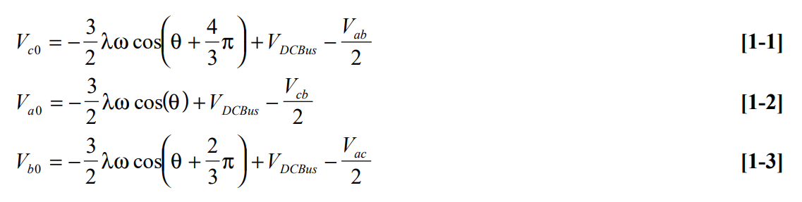
From these equations it is apparent that the back EMF waveform is a non-linear function of both velocity and position. In the next section an extended Kalman estimator is developed which estimates both position and velocity based on these non-linear measurements.

The Kalman Estimator

Given a discrete time stochastic state space description of a system [1-4] and an observation model [1-5], where Φ, Γ and H in equations [1-4] and [1-5] have their usual state space interpretation and where ω_k and υ_k and denote process noise and measurement noise sequences respectively, then an estimate of the states of the plant is given by equation [1-7] where K_k is the Kalman gain described by equations [1-8], [1-9] and [1-10]. These equations combine to form the algebraic Riccati equation. These process and measurement noise sequences are assumed to be uncorrelated, with zero mean and normal distributions. Formally these noises can be mathematically described using equations [1-11], [1-12] and [1-13]. The matrices Q_k and R_k are defined as positive definite symmetric matrices [Kalman 60], [Gelb 74], [Grimble 88], [Haykin 89].

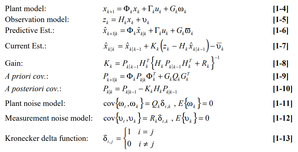
In the case of a non-linear plant or measurement models such a steady state solution does not exist in the general case. Consequently the algebraic Riccati equation and estimator gains must be solved in real time.

The Extended Kalman Estimator

For the Extended Kalman filter the gaussian signal model equations [1-4] and [1-5] are replaced with nonlinear signal models described by equation [1-14] and [1-15], where Φ(·) and Γ(·) are nonlinear functions and G(·) is, in general, non-constant. In this particular application only the observation signal model is nonlinear, consequently for this problem only equation [1-15] is required.

In the Extended Kalman filter design the nonlinear gaussian signal model is linearised about the most recent state estimate. This Extended Kalman filter is a suboptimal filter design because the linearised signal model is an approximation of the real signal model. In this case the suboptimality of the Extended Kalman filter exists only with the choice of a reference trajectory for the innovation sequence. For a concise definition of the Extended Kalman filter see [Jazwinski 70, Theorem 8.1], [Anderson 79] and [Mendel 87]. In the Extended Kalman construction the nonlinear function if sufficiently smooth is expanded in a Taylor series expansion about the most recent estimate. This ensures that the available linear approximation of the observation model is the best available approximation. Hence the reference trajectory is the best available trajectory. Equation [1-16] describes the first two terms of a Taylor series expansion for the nonlinear function, where H in equation [1-16] is a Jacobian matrix defined by equation [1-17].

By redefining the a priori and a posteriori error covariance the estimator problem can be redefined in terms of the linearised observation model. Equations [1-18] to [1-24] define the Extended Kalman filter for a gaussian signal model with a nonlinear observation model.

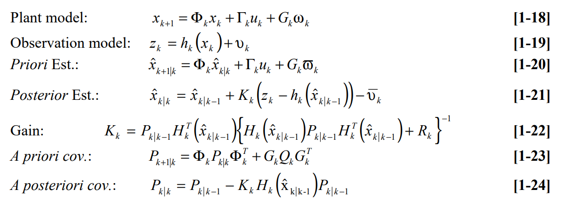
The overall structure of the Extended Kalman filter remains the same as that of the Linear Kalman filter. However from equation [1-22] it is immediately apparent that the EKF gains are a function of the most recent estimate.

State Equation Definition

In this paper the plant models that are used are based on Newtonian models for position and velocity. These models are generic insofar as no motor dynamics parameters are required. Other models are available which make use of the motor mechanical and electrical parameters. These in general will improve the response and convergence times of the estimator. Furthermore other states can be estimated such as disturbance torque, DC Bus voltage and the motor’s back EMF constant. These models will however introduce added complexity, which is not necessary in most applications. The algorithm presented here is the least common denominator for a sensorless algorithm.

Define the following states and plant model:

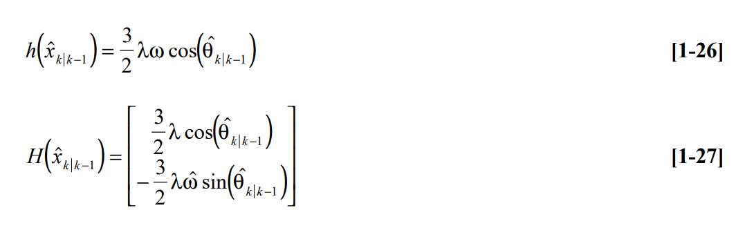
For a sinusoidal wound motor, define the following measurement equation based on equation [1-2] and corresponding Jacobian matrix.

Tuning

The Kalman filer is a stochastic filter. Its bandwidth is defined by the stochastic processes that couple into the plant model. Recall that ω_k and υ_k denote process noise and measurement noise sequences respectively in equations [1-4] and [1-5], from which plant and measurement covariance matrices are derived, [1-12] and [1-11].

The two matrices [1-12] and [1-11] set the filter bandwidth in the classical sense. In the case of a Kalman filter the plant and measurement covariance typically are known. In the case of a Kalman estimator the plant and measurement covariance also define the estimator bandwidth. Filtering the measurement and process noise is often secondary to the convergence speed of the estimator [Kettle 94]. This is especially true in robust applications where the estimator is used in the feedback path of a closed loop system. In these applications the covariance matrices often lose their stochastic origins and simply become tuning parameters.

Throughout this paper references to estimator ‘bandwidth’ are qualified with ‘in the classical sense’. Unlike a conventional estimator / filter the time varying Kalman estimator is a stochastic filter. Its bandwidth is a time varying parameter which is a function of the measurement uncertainty. This becomes significant when designing a robust controller where this estimator forms the feedback path. For a robust controller design it is necessary to ensure that the estimator ‘bandwidth’ is ‘faster’ than that of the controller [Kettle 94],[Kettle 96] [Kettle 97].

The Algorithm Implementation

The Extended Kalman estimator defined by equations [1-18] to [1-24] can be implemented as a series of matrix multiplication’s. However given that some of the matrices are symmetric and several elements are either zeros or one, it is often more efficient to expand these equations into their simplest form.

Define the following matrix notation:

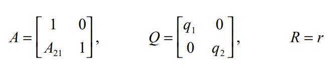
Substitute the above definitions into [1-22] and simplify:

Likewise expand [1-23] and [1-24].

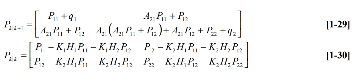
Equation [1-20] may be reduced a linear equation:

Likewise [1-21] may be reduced to:

Expermental Results

Figure [1-5] and [1-6] depict the phase voltages for a trapezoidally driven motor, where the high side devices are clamped and the low side devices are chopped. Four distinct states can be clearly identified in these plots, high side clamping, flyback, back EMF and low side chopping. The lower portion of figure [1-6] represents a concatenation of the back EMF state samples synchronized with the PWM ripple. This waveform corresponds to the measurement equation used in the Kalman estimator.

Depending on the inactive phase either [1-2], [1-3] or [1-1] will correspond to the sampled data.

Table [1-1] EKE Algorithm.

Equation No.	Execution Time	No. of Instr.
[1-29].	0.90μs	18
[1-31].	0.35μs	7
Detect flyback,	1.00μs	20
[1-26]&[1-27].	3.85μs	≈77
[1-28].	4.25μs	≈85
[1-32].	1.00μs	20
[1-30].	1.55μs	31
Total	12.9μs	≈258

Figure [1-7] depicts the estimated concatenated back EMF data and the corresponding position estimate. The lower portion of the figure corresponds to a position reference measurement obtained from a sinusoidal resolver.

This estimator is typically used in conjunction with a linear quadratic controller to close a velocity loop. The algorithm does however have an inherent limitation. At low speeds the signal to noise ratio for the back emf data is typically quite poor. Consequently the state estimates are equally poor. To start the motor it is necessary to control it in an open loop configuration until sufficient back emf has been generated. The algorithm presented in this paper will converge to a good estimate in approximately 60 electrical degrees. For applications such as compressors, fans or pumps where the initial load dynamics are deterministic and low speed operation is not required such an algorithm is well suited.

Conclusion

The sensorless control algorithm presented in this paper has many applications in appliances, and in automotive and industrial control. With the advent of fast low cost DSP motor controllers such as the ADMC330, the cost-effective realization of such an estimation algorithm is now a reality. These algorithms provide far superior performance over the classical zero crossing sensorless approach. Indeed the availability of instantaneous position, velocity and disturbance torque information greatly improves the efficiency, and robustness of the system, while decreasing the acoustic noise.

This particular paper only deals with the estimator portion of the controller. When integrated with a LQ (linear quadratic) controller, the resulting LQG (linear quadratic gaussian) controller forms the most optimal controller in the gaussian sense. The LQG theory provides an integrated knowledge base for powerful controller design topography. With the increasing computational bandwidth made available through the use of DSPs, elaborate and sophisticated control schemes such as LQG enable the designer to develop reduced sensor / sensorless control schemes. Moreover, controller states, such as disturbance torque which are not readily measured, can now be estimated and thus controlled. [Kettle 97], [Kettle 96], [Kettle 94].

The estimation portion of the algorithm presented was developed for and implemented on the Analog Devices ADMC330 DSP motor controller. The algorithm requires approximately 500 DSP instructions and executes in approximately 13µs, utilizing approximately 30% of the available computation resources of the DSP controller.

References

[Anderson 79] Optimal Filtering. Brian D.O. Anderson and John B. Moore, Prentice-Hill 1979.

[Gelb 74] Applied Optimal Estimation. Edited by Arthur Gelb. Massachusetts Institute of Technology. 1974.

[Grimble 88a] Optimal Control and Stochastic Estimation Volume 1. Michael J. Grimble and Michael A. Johnson. John Wiley & Son 1988.

[Grimble 88b] Optimal Control and Stochastic Estimation Volume 2. Michael J. Grimble and Michael A. Johnson. John Wiley & Son 1988.

[Jazwinski 70] Stochastic Processes and Filtering Theory. Andrew H. Jazwinski. Academic Press 1970.

[Kalman 60] A New Approach to Linear Filtering and Prediction Problems. R.E. Kalman Trans. ASME. Journal of Basic Eng., Mar 1960, Vol. 82, pp 34-45.

[Kettle 97] A DSP based Robust Optimal Servo Motor controller. P J. Kettle, A Murray, A Holohan. Preceedings from EPE’97, September 97 pp 3.876-3.881.

[Kettle 96] Robust Optimal Servo Motor controller design. P J. Kettle, A Murray, A Holohan. Preceedings from ICSPAT 96, October 96 Boston MA pp 1196-1203.

[Kettle 94], “Robust-Optimal Control for a Servo Motor”. PhD Dissertation Dublin City University, School of Electronic Engineering 1994.

[Mendel 71] Computational Requirements for a Discrete Kalman Filter. Jerry M. Mendel. IEEE Transactions On Automatic Control, Vol. AC-16, No. 6 December 1971. pp 748-758.

[Mendel 87] Lessons in Digital Estimation Theory. Jerry M. Mendel. Prentice-Hall 1987.

[Murray 96] Towards a single chip DSP based motor control solution, A. Murray and P. Kettle, Proceedings PCIM’96, Nurenberg, May 1996, pp.315-326

[Vaughan 70] A Nonrecursive Algebraic Solution for the Discrete Riccati Equation. David R. Vaughan. IEEE Transactions on Automatic Control, Oct. 1970, Vol. AC-15 pp. 597-599.

关于作者

Paul Kettle

Aengus Murray

Aengus Murray 是ADI公司汽车、能源和传感器部门的电机和电源控制应用经理。他负责工业电机和电源控制的整个ADI信号链产品。Murray拥有爱尔兰都柏林大学电气工程学士和博士学位。他在功率电子行业拥有超过30年的丰富经验，曾先后在Rectifier、Kollmorgen Industrial Drives和都柏林城市大学工作。

Finbarr Moynihan